Linear_Model_Example
Zhuoran (Angela) Yu
2025-11-04
Source:vignettes/Linear_Model_Example.Rmd
Linear_Model_Example.RmdThe example here is to use simulated data to construct the
simultaneous outer and inner confidence regions (SCRs) from simultaneous
confidence bands (SCB) using linear regression.
SCoRES::SCB_linear_outcome() function uses a non-parametric
bootstrap algorithm to construct the SCB in linear regression. The
argument df_fit specifies a data frame containing the
training design matrix used to fit the linear model, while
grid_df defines the mean outcome for which simultaneous
confidence bands (SCB) are constructed. Use argument model
to specify the formula used for fitting the linear model.
SCBs for Mean Outcome of Linear Model
In the following example, we use a linear regression to estimate the simultaneous confidence band (SCB) for the mean outcome, with modeling equation as follows:
We establish simultaneous confidence bands for the expected response surface , with the independent variables and discretized into 100 equidistant points over the domain .
library(SCoRES)
set.seed(262)
# generate simulated data
x1 <- rnorm(100)
x2 <- rnorm(100)
epsilon <- rnorm(100,0,sqrt(2))
y <- -1 + x1 + 0.5 * x1^2 - 1.1 * x1^3 - 0.5 * x2 + 0.8 * x2^2 - 1.1 * x2^3 + epsilon
df <- data.frame(x1 = x1, x2 = x2, y = y)
grid <- data.frame(x1 = seq(-1, 1, length.out = 100), x2 = seq(-1, 1, length.out = 100))
# fit the linear regression model and obtain the SCB for y
model <- "y ~ x1 + I(x1^2) + I(x1^3) + x2 + I(x2^2) + I(x2^3)"
results <- SCB_linear_outcome(df_fit = df, model = model, grid_df = grid)
The levels = c(-0.3, 0, 0.3) argument specifies a set of
thresholds, and SCoRES::plot_cs() function estimates
multiple inverse upper excursion sets corresponding to these thresholds,
and plots the estimated inverse regions, the inner confidence regions,
and the outer confidence regions.
results <- tibble::as_tibble(results)
suppressWarnings(plot_cs(results,
        levels = c(-0.3, 0, 0.3),
        x = seq(-1, 1, length.out = 100),
        mu_hat = results$Mean,
        xlab = "x1",
        ylab = "y",
        level_label = T,
        min.size = 40,
        palette = "Spectral",
        color_level_label = "black"))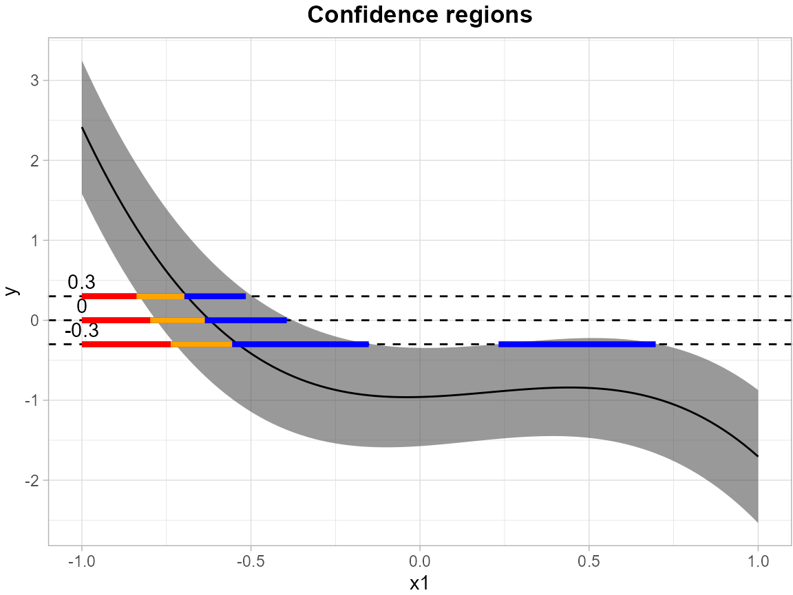
In the following example, we establish simultaneous confidence bands for the expected response surface , with the independent variable discretized into 100 equidistant points over the domain .
x1 <- rnorm(100)
x2 <- rnorm(100)
epsilon <- rnorm(100,0,sqrt(2))
y <- -1 + x1 + 0.5 * x1^2 - 1.1 * x1^3 - 0.5 * x2 + 0.8 * x2^2 - 1.1 * x2^3 + epsilon
df <- data.frame(x1 = x1, x2 = x2, y = y)
# fit the linear regression model and obtain the SCB for y
model <- "y ~ x1 + I(x1^2) + I(x1^3) + x2 + I(x2^2) + I(x2^3)"
grid <- data.frame(x2 = seq(-1, 1, length.out = 100))
results <- SCB_linear_outcome(df_fit = df, model = model, grid_df = grid)
The levels = c(-1.5, -1.0, -0.5) argument specifies a
set of thresholds, and SCoRES::plot_cs() function estimates
multiple inverse upper excursion sets corresponding to these thresholds,
and plots the estimated inverse regions, the inner confidence regions,
and the outer confidence regions.
results <- tibble::as_tibble(results)
suppressWarnings(plot_cs(results,
        levels = c(-1.5, -1.0, -0.5),
        x = seq(-1, 1, length.out = 100),
        mu_hat = results$Mean,
        xlab = "x2",
        ylab = "y",
        level_label = T,
        min.size = 40,
        palette = "Spectral",
        color_level_label = "black"))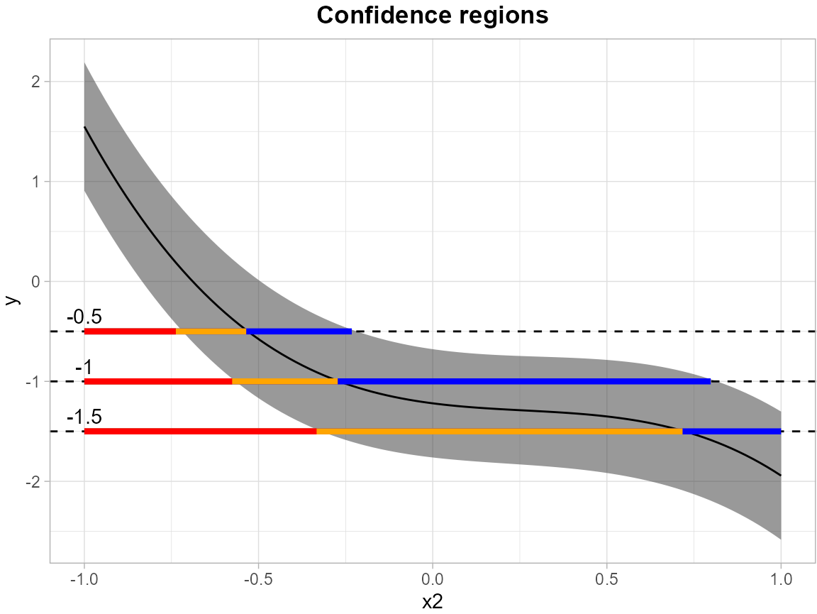
SCBs for Mean Outcome of Logistic Model
In addition to linear regression, SCoRES also
providesSCoRES::SCB_logistic_outcome() for estimating the
SCB for outcome of logistic regression.
Here, we use a similar model structure with logistic regression to estimate the simultaneous confidence band (SCB) for the outcome probability, with modeling equation as follows:
We establish simultaneous confidence bands for the expected response surface , with the independent variables and discretized into 100 equidistant points over the domain .
# generate simulated data
x1 <- rnorm(100)
x2 <- rnorm(100)
mu <- -1 + x1 + 0.5 * x1^2 - 1.1 * x1^3 - 0.5 * x2 + 0.8 * x2^2 - 1.1 * x2^3
p <- expit(mu)
y <- rbinom(100, size = 1, prob = p)
df <- data.frame(x1 = x1, x2 = x2, y = y)
grid <- data.frame(x1 = seq(-1, 1, length.out = 100), x2 = seq(-1, 1, length.out = 100))
# fit the logistic regression model and obtain the SCB for y
model <- "y ~ x1 + I(x1^2) + I(x1^3) + x2 + I(x2^2) + I(x2^3)"
results <- SCB_logistic_outcome(df_fit = df, model = model, grid_df = grid)
Likewise, the levels = c(0.3, 0.4, 0.5) argument
specifies a set of thresholds, and SCoRES::plot_cs()
function estimates multiple inverse upper excursion sets corresponding
to these thresholds, and plot the estimated inverse region, the inner
confidence region, and the outer confidence region.
results <- tibble::as_tibble(results)
plot_cs(results,
        levels = c(0.3, 0.4, 0.5),
        x = seq(-1, 1, length.out = 100),
        mu_hat = results$Mean,
        xlab = "x1",
        ylab = "y",
        level_label = T,
        min.size = 40,
        palette = "Spectral",
        color_level_label = "black")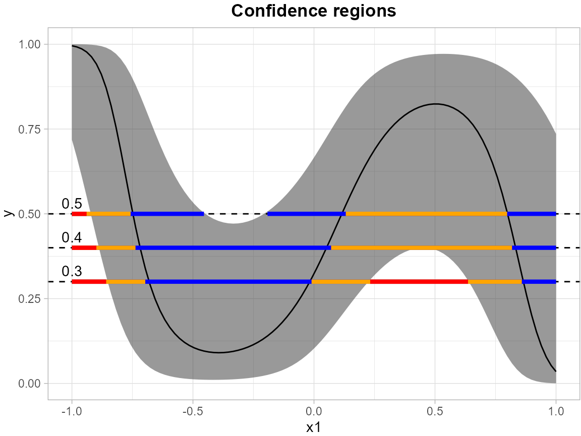
SCBs for Coefficients of Linear/Logistic Model
Besides, SCoRES::SCB_regression_coef can estimate the
SCB for every coefficient in the linear/logistic model.
Here, we use a linear regression model with 50 coefficients in total to estimate the simultaneous confidence band (SCB) for all coefficients and the intercept, with modeling equation as follows: where .
library(MASS)
# generate simulated data
M <- 50
rho <- 0.4
n <- 500
beta <- rnorm(M, mean = 0, sd = 1)
Sigma <- outer(1:M, 1:M, function(i, j) rho^abs(i - j))
X <- MASS::mvrnorm(n = n, mu = rep(0, M), Sigma = Sigma)
epsilon <- rnorm(n, mean = 0, sd = 1)
y <- X %*% beta + epsilon
df <- as.data.frame(X)
names(df) <- paste0(1:M)
df$y <- as.vector(y)
# fit the linear regression model and obtain the SCB for all betas
model <- "y ~ ."
results <- SCB_regression_coef(df, model)
Likewise, the levels = c(-2, -0.5, -0.1, 0.2) argument
specifies a set of thresholds, and SCoRES::plot_cs()
function estimates multiple inverse upper excursion sets corresponding
to these thresholds, and plots the estimated inverse regions, the inner
confidence regions, and the outer confidence regions.
results <- tibble::as_tibble(results)
plot_cs(results,
        levels = c(-2, -0.5, -0.1, 0.2),
        x = c("intercept", as.character(1:50)),
        mu_hat = results$Mean,
        xlab = "Coefficients",
        ylab = "SCBs for Coefficients",
        level_label = T,
        min.size = 40,
        palette = "Spectral",
        color_level_label = "black")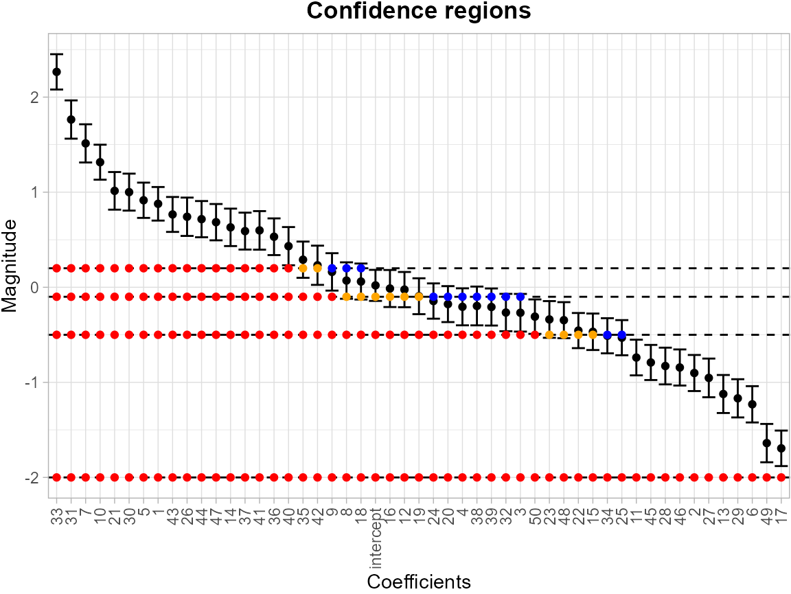
Users can also compute the SCB for any linear combination of these
coefficients by specifying a weight vector of the same length as the
coefficient vector. This can be done by using
SCoRES::SCB_regression_outcome(), and specifying the linear
combination through w. For example, suppose we want to
calculate the SCB for the linear combination
for model:
:
x1 <- rnorm(100)
x2 <- rnorm(100)
epsilon <- rnorm(100,0,sqrt(2))
y <- -1 + x1 + 0.5 * x1^2 - 1.1 * x1^3 - 0.5 * x2 + 0.8 * x2^2 - 1.1 * x2^3 + epsilon
df <- data.frame(x1 = x1, x2 = x2, y = y)
grid <- data.frame(x1 = seq(-1, 1, length.out = 100), x2 = seq(-1, 1, length.out = 100))
# fit the linear regression model and obtain the SCB for y
model <- "y ~ x1 + I(x1^2) + I(x1^3) + x2 + I(x2^2) + I(x2^3)"
w <- matrix(c(0, 1, 1, 1, 0, 0, 0), ncol = 7)

SCB_regression_outcome(df_fit = df, model = model,
                       grid_df = grid, n_boot = 50, alpha = 0.1,
                       fitted = FALSE, w = w)
#>            scb_low      Mean   scb_up
#> scb_low -0.4971322 0.3964766 1.290085
In the following example, we load ipad dataset, and
establish simultaneous confidence bands for all the coefficients and the
intercept in the model fitted. Here, we set log(t_mmr1) as
the outcome, and include all variables from Pupillography,
Tablet (task metrics) and Cardiovascular as
predictors.
library(SCoRES)
library(dplyr)
library(ggplot2)
set.seed(262)
data(ipad)
df <- ipad %>%
  filter(t_mmr1 > 0) %>%
  select(p_fpc1, p_fpc2, p_fpc3, p_fpc4, p_fpc5, p_fpc6,
         p_PMC_pctChg, p_auc, t_mmr1,
         i_prop_false_timeout, i_prop_failed1, i_prop_failed2,
         i_judgement_time1, i_judgement_time2, i_time_outside_reticle,
         i_time_on_edge, i_prop_hit, i_correct_reaction2,
         i_reaction_time_max2, i_reaction_time2, i_rep_shapes12,
         i_rep_shapes34, i_memory_time12, i_memory_time34,
         i_composite_score, h_hr, h_dbp, h_sbp, recent_smoke) %>%
  mutate(log_tmmr1 = log(t_mmr1))
df_lin <- df %>%
  select(-recent_smoke, -t_mmr1)
# fit the linear regression model and obtain the SCB for y
model_lin <- "log_tmmr1 ~ ."
results <- SCB_regression_coef(df_fit = df_lin, model = model_lin)
The levels = c(0.2, 0.3, 0.4) argument specifies a set
of thresholds, and SCoRES::plot_cs() function estimates
multiple inverse upper excursion sets corresponding to these thresholds,
and plot the estimated inverse region, the inner confidence region, and
the outer confidence region. Here, for illustration, we filter out the
SCB for intercept.
results <- tibble::as_tibble(results[-1, ])
suppressWarnings(plot_cs(results,
        levels = c(0.2, 0.3, 0.4),
        x = c(names(df_lin)[1:(length(names(df_lin))-1)]),
        mu_hat = results$Mean,
        xlab = "",
        ylab = "",
        level_label = T,
        min.size = 40,
        palette = "Spectral",
        color_level_label = "black"))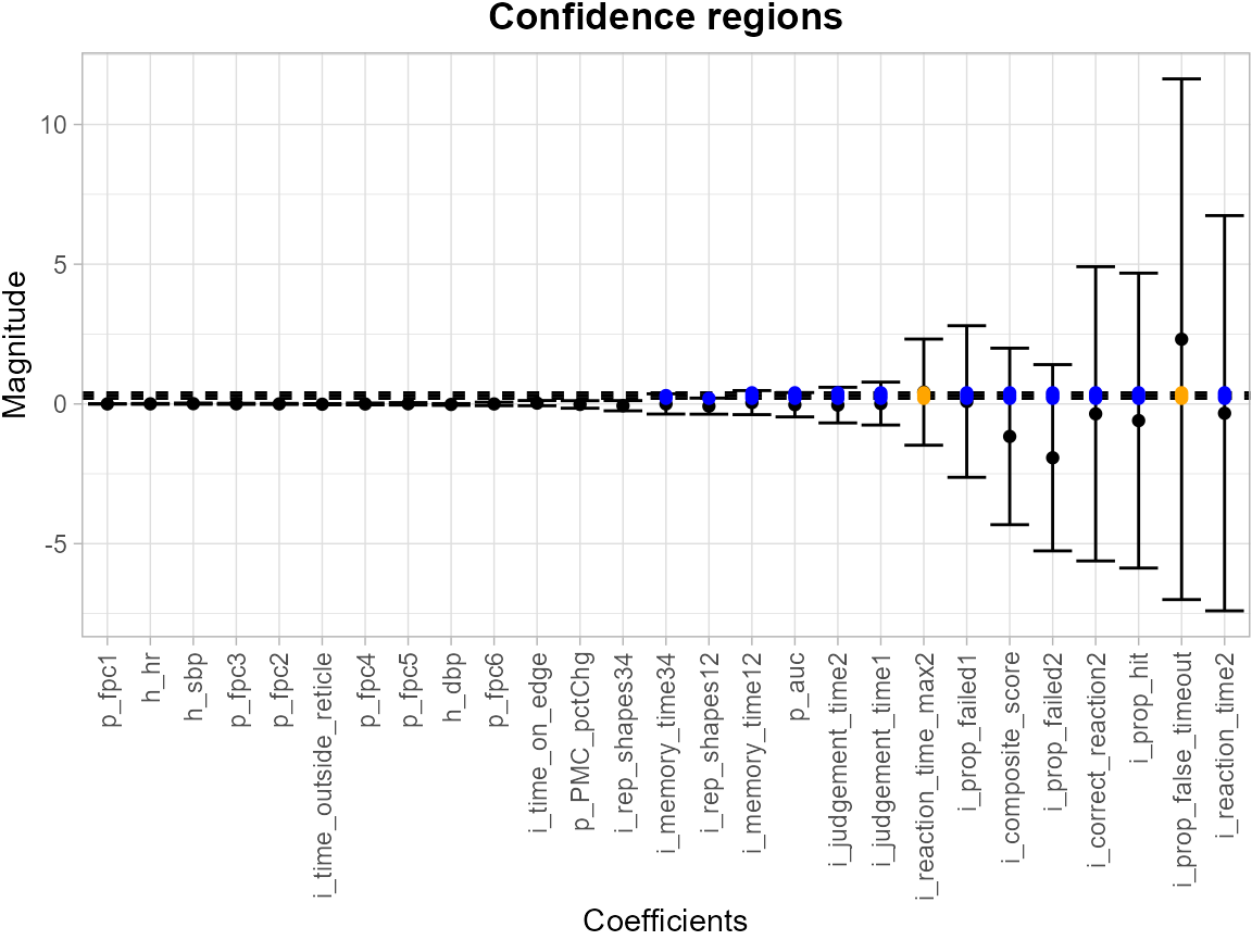
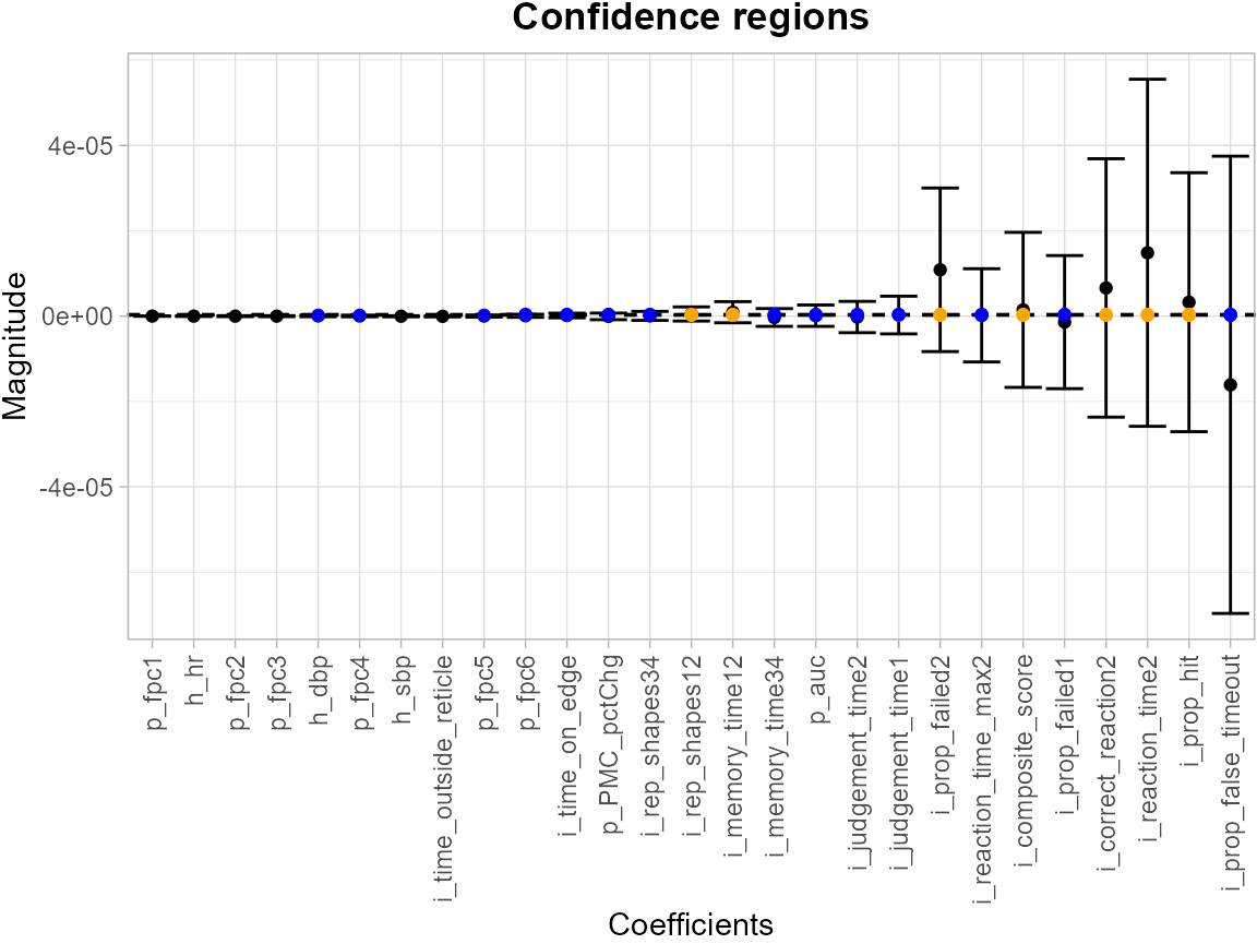
We fit a logistic model with recent_smoke as outcome
with the same predictors in linear regression model, and obtain SCBs for
all coefficients and the intercept.
df_log <- df %>%
  select(-t_mmr1, -log_tmmr1)
# fit the logistic regression model and obtain the SCB for y
model_log <- "recent_smoke ~ ."
results <- SCB_regression_coef(df_fit = df_log, model = model_log, type = "logistic")
The levels = c(2e-07, 3e-07, 4e-07) argument specifies a
set of thresholds, and SCoRES::plot_cs() function estimates
multiple inverse upper excursion sets corresponding to these thresholds,
and plots the estimated inverse regions, the inner confidence regions,
and the outer confidence regions. Here, for illustration, we filter out
the SCB for intercept.
results <- tibble::as_tibble(results[-1, ])
suppressWarnings(plot_cs(results,
        levels = c(2e-07, 3e-07, 4e-07),
        x = c(names(df_log)[1:(length(names(df_log))-1)]),
        mu_hat = results$Mean,
        xlab = "",
        ylab = "",
        level_label = T,
        min.size = 40,
        palette = "Spectral",
        color_level_label = "black"))