Functional_Data_Example
Zhuoran (Angela) Yu
2025-11-04
Source:vignettes/Functional_Data_Example.Rmd
Functional_Data_Example.RmdOverview
The example here is to use pupil functional data to construct the simultaneous outer and inner confidence regions (SCRs) from simultaneous confidence bands (SCBs) using Function-on-Scalar Regression (FoSR).
The pupil dataset contains repeated measures of percent change over time for multiple subjects under two user categories (use: 1 and no use: 0). It contains both user and non-user groups, multiple time points, and several covariates, including age, gender, BMI, and alcohol consumption.
Before calculating the SCBs, we first process pupil data by fitting a
mean GAM model, extracting residuals and performing FPCA using
SCoRES::prepare_pupil_fpca(), the function will return an
enhanced dataset that includes the FPCA-derived basis scores (Phi1,
Phi2, Phi3, Phi4) for Function-on-Scalar Regression (FoSR) analysis.
Following the FPCA-based data augmentation, we fit a FoSR model using
mgcv::bam(), which allows efficient estimation of
Generalized Additive Mixed Models (GAMMs). The model formula is designed
to capture both population-level smooth trends and subject-specific
functional variation.
The response here is percent_change. Time variable t is seconds, and the covariate is use, which is a binary indicator (1:use, 0:no use).
The function-on-scalar regression model is
pupil_fpca <- SCoRES::prepare_pupil_fpca(pupil)
fosr_mod <- mgcv::bam(percent_change ~ s(seconds, k=30, bs="cr") +
            s(seconds, by = use, k=30, bs = "cr") +
            s(id, by = Phi1, bs="re") +
            s(id, by = Phi2, bs="re") +
            s(id, by = Phi3, bs="re") +
            s(id, by = Phi4, bs="re"),
            method = "fREML", data = pupil_fpca, discrete = TRUE)
After obtaining the FoSR object fosr_mod, the
simultaneous confidence bands (SCBs) can be constructed through
SCoRES::SCB_functional_outcome using pre-specified methods.
The SCoRES package provides two options for calculating simultaneous
confidence bands (SCBs), specified via the method argument:
cma: Correlation and Multiplicity Adjusted (CMA) confidence
bands via parametric approach from Crainiceanu et
al. (2024). multiplier: Dense confidence bands via
Multiplier-t Bootstrap method from Telschow &
Schwartzman (2022). Use subset to specify the names
of grouping variables to analyze. The input data should have numerical
binary 0/1 values for all scalar group variables. Here, we analyze the
user group by specifying subset = c("use = 1"). Use
fitted to specify the object for SCB estimation. If
fitted = TRUE, SCoRES::SCB_functional_outcome
will construct the SCB for the fitted mean outcome function. If
fitted = FALSE, SCoRES::SCB_functional_outcome
will construct the SCB for the fitted parameter function. For
cma option, users are required to provide a functional
regression object through argument object. For
multiplier option, users also need to provide input for
object. If object = NULL, the function will
only output the SCB for an overall mean outcome function regardless of
the group specified.
Here, we estimate SCBs using both options separately for the mean outcome Y(t) of user’s group:
In the multiplier bootstrap procedure, SCoRES supports
three types of multiplier distributions, which is specified by
weights:
-
"rademacher": with equal probability -
"gaussian": -
"mammen": A two-point distribution with mean zero and variance one (see Mammen, 1993)
Default is rademacher.
Two options are available for estimating the standard error
,
which is specified by method_SD:
“regular” (empirical standard error based on residuals):
“t” (bootstrap second moment-based estimator):
Default is t.
For mathematical details, see vignette Methods.
Correlation and Multiplicity Adjusted (CMA) Confidence Bands
SCB for Mean Outcome Function
The code below visualizes the simultaneous outer and inner regions
derived from SCB results using the SCoRES::plot_cs()
function. The results object is first converted to a tibble
for easier manipulation.
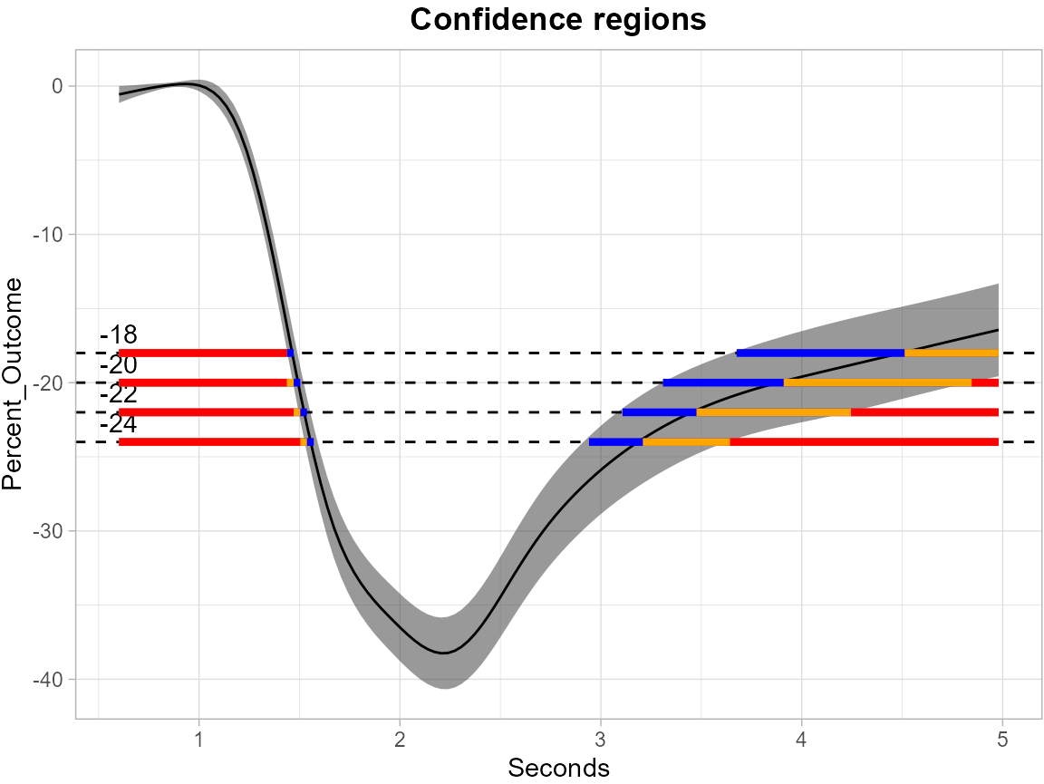
The levels = c(-18, -20, -22, -24) argument specifies a
set of thresholds, and SCoRES::plot_cs() function estimates
multiple inverse upper excursion sets corresponding to these thresholds,
and plots the estimated inverse regions, the inner confidence regions,
and the outer confidence regions.
# CMA approach
results_pupil_cma <- SCoRES::SCB_functional_outcome(
                                          data_df = pupil,
                                          object = fosr_mod,
                                          method = "cma",
                                          fitted = TRUE,
                                          alpha = 0.05,
                                          outcome = "percent_change",
                                          domain = "seconds",
                                          subset = c("use = 1"),
                                          id = "id")

results_pupil_cma <- tibble::as_tibble(results_pupil_cma)
plot_cs(results_pupil_cma,
        levels = c(-18, -20, -22, -24),
        x = results_pupil_cma$domain,
        mu_hat = results_pupil_cma$mu_hat,
        xlab = "Seconds",
        ylab = "Percent_Outcome",
        level_label = T,
        min.size = 40,
        palette = "Spectral",
        color_level_label = "black")
The plot demonstrates how to use SCBs to find regions of time where the estimated mean is greater than or equal to the four levels -18, -20, -22 and -24 for pupil data. The gray shaded area is the 95% SCB, the solid black line is the estimated mean. The red horizontal line shows the inner confidence regions (where the lower SCB is greater than the corresponding level) that are contained in the estimated inverse region represented by the union of the yellow and red horizontal line (where the estimated mean is greater than the corresponding levels); the outer confidence regions are the union of the blue, yellow and red line (where the upper SCB is greater than the corresponding levels) and contain both the estimated inverse regions and the inner confidence regions.
SCB for Coefficient Function
The next plot shows the SCB for the coefficient function for the use group, and the corresponding SCRs based on specified levels.
#CMA approach for parameter function
results_pupil_cma_para <- SCoRES::SCB_functional_outcome(
                                          data_df = pupil,
                                          object = fosr_mod,
                                          method = "cma",
                                          fitted = FALSE,
                                          alpha = 0.05,
                                          outcome = "percent_change",
                                          domain = "seconds",
                                          subset = c("use = 1"),
                                          id = "id")

results_pupil_cma_para <- tibble::as_tibble(results_pupil_cma_para)
plot_cs(results_pupil_cma_para,
        levels = c(4.5, 5, 5.5, 6),
        x = results_pupil_cma_para$domain,
        mu_hat = results_pupil_cma_para$mu_hat,
        xlab = "Seconds",
        ylab = "Percent_Outcome",
        level_label = T,
        min.size = 40,
        palette = "Spectral",
        color_level_label = "black")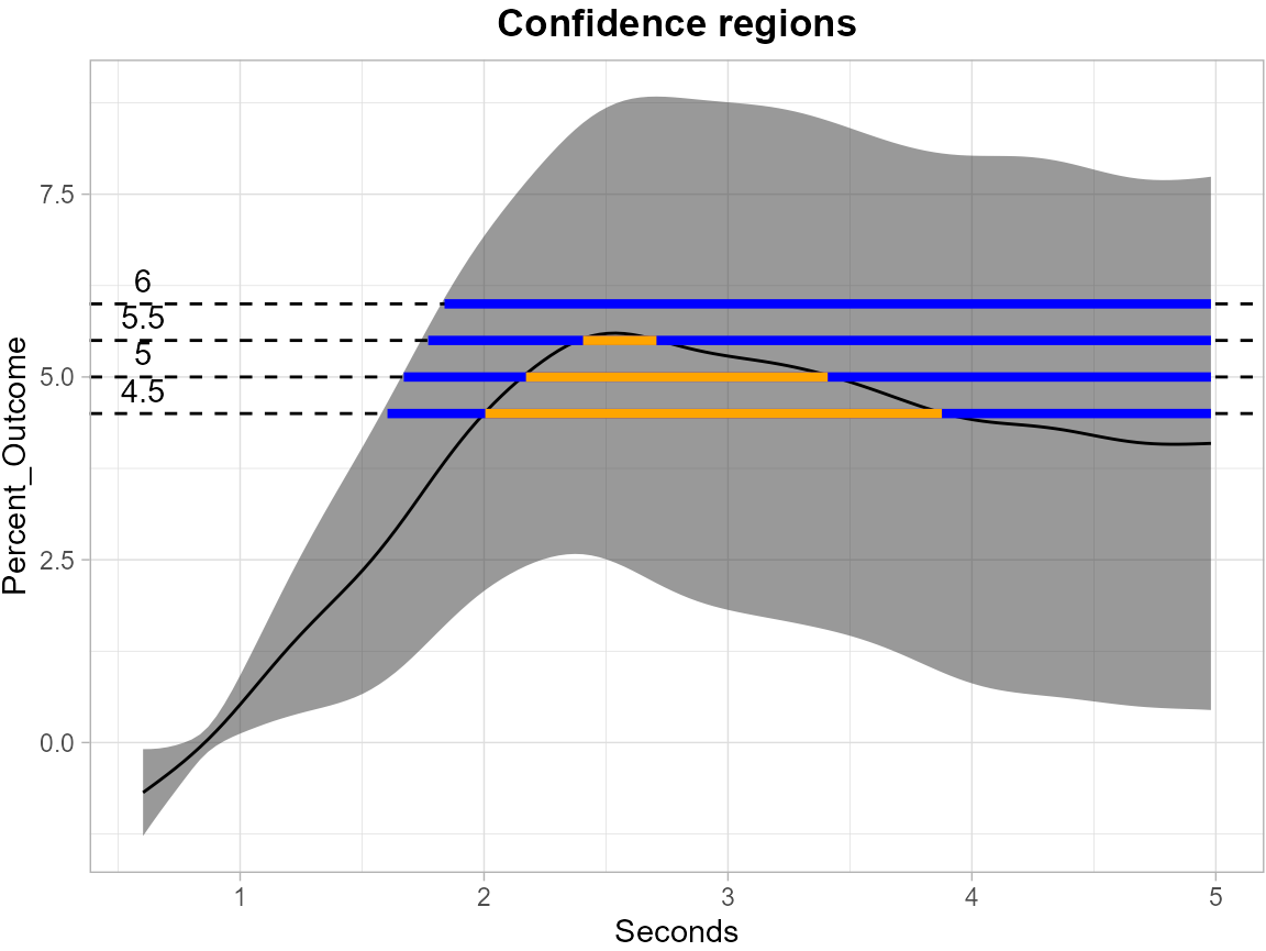
Multiplier-t Bootstrap Confidence Bands
SCB for Mean Outcome Function
The following plots show the results of multiplier bootstrap. The
first one displays the SCB for mean outcome function for the use group,
while the second one is for the coefficient function of the use group.
All possible NA’s are imputed using
refund::fpca.face().
# Multiplier-t Bootstrap
results_pupil_multiplier <- SCoRES::SCB_functional_outcome(
                                          data_df = pupil,
                                          object = fosr_mod,
                                          method = "multiplier",
                                          fitted = TRUE,
                                          alpha = 0.05,
                                          outcome = "percent_change",
                                          domain = "seconds",
                                          subset = c("use = 1"),
                                          id = "id")

results_pupil_multiplier <- tibble::as_tibble(results_pupil_multiplier)
plot_cs(results_pupil_multiplier,
        levels = c(-18, -20, -22, -24),
        x = results_pupil_multiplier$domain,
        mu_hat = results_pupil_multiplier$mu_hat,
        xlab = "Seconds",
        ylab = "Percent_Outcome",
        level_label = T,
        min.size = 40,
        palette = "Spectral",
        color_level_label = "black")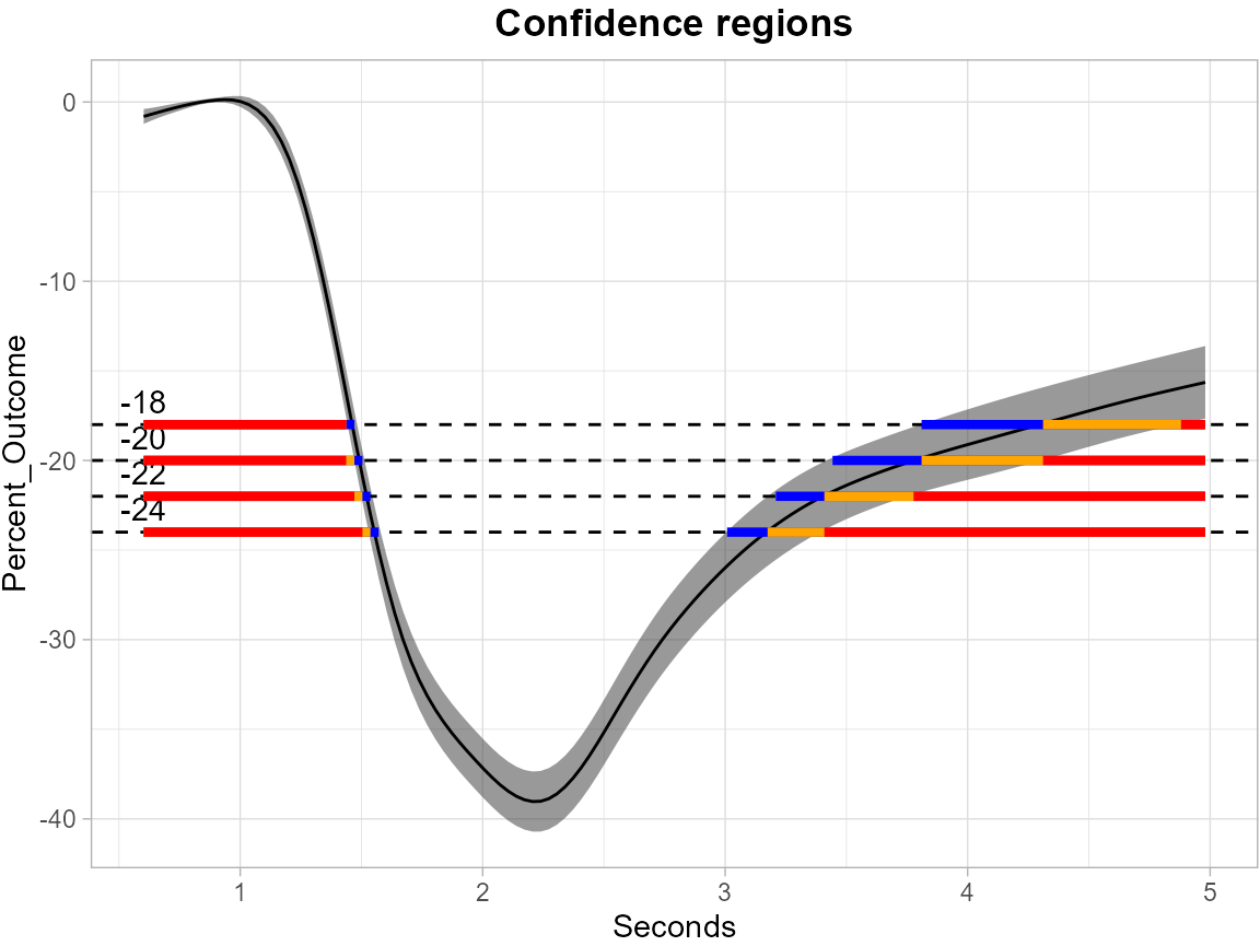
SCB for Coefficient Function
results_pupil_multiplier_para <- SCoRES::SCB_functional_outcome(
                                          data_df = pupil,
                                          object = fosr_mod,
                                          method = "multiplier",
                                          fitted = FALSE,
                                          alpha = 0.05,
                                          outcome = "percent_change",
                                          domain = "seconds",
                                          subset = c("use = 1"),
                                          id = "id")

results_pupil_multiplier_para <- tibble::as_tibble(results_pupil_multiplier_para)
plot_cs(results_pupil_multiplier_para,
        levels = c(4.5, 5, 5.5, 6),
        x = results_pupil_multiplier_para$domain,
        mu_hat = results_pupil_multiplier_para$mu_hat,
        xlab = "Seconds",
        ylab = "Percent_Outcome",
        level_label = T,
        min.size = 40,
        palette = "Spectral",
        color_level_label = "black")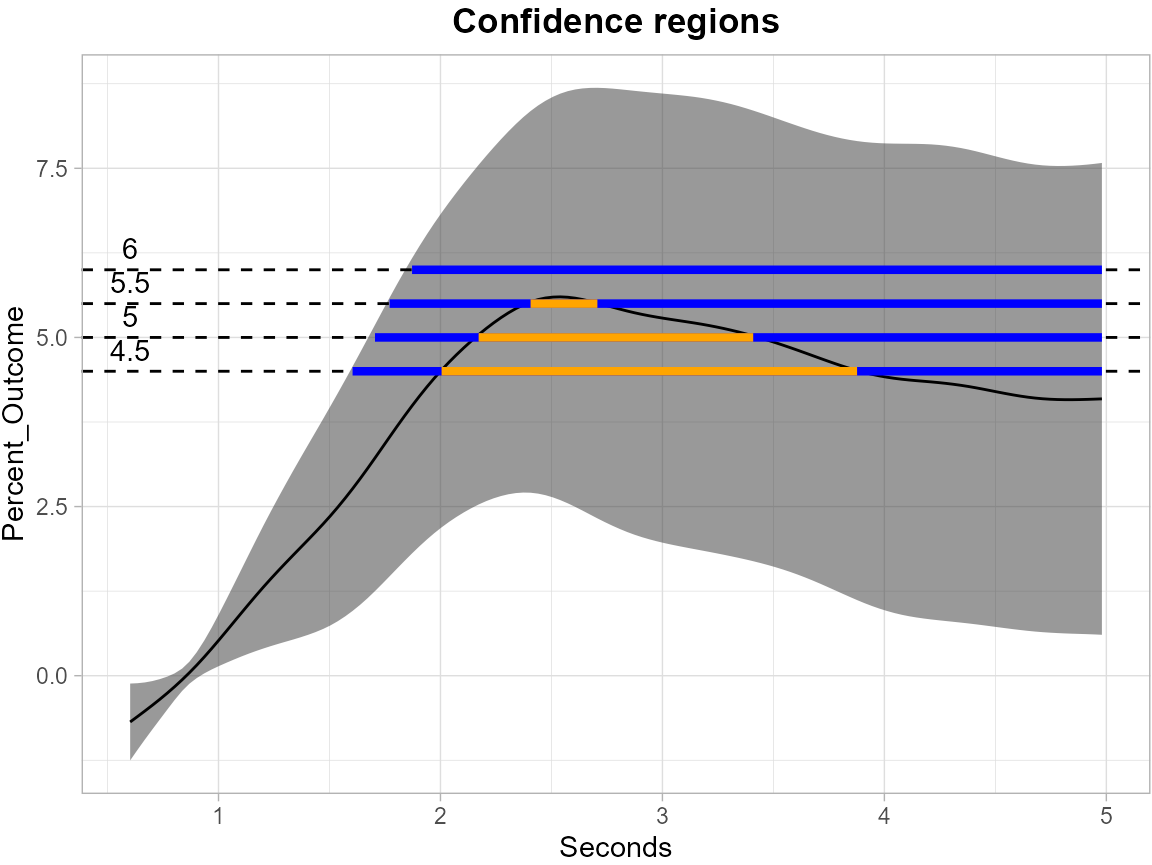
The following plot displays the SCB and the corresponding SCRs of specified levels for the overall mean outcome function. The solid black line represents the sample mean.
results_pupil_multiplier_overall <- SCoRES::SCB_functional_outcome(
                                          data_df = pupil,
                                          method = "multiplier",
                                          fitted = TRUE,
                                          alpha = 0.05,
                                          outcome = "percent_change",
                                          domain = "seconds",
                                          subset = c("use = 1"),
                                          id = "id")
#> [1] "No Functional Regression Object provided, will only compute an overall SCB for the outcome regardless of the group specified."

results_pupil_multiplier_overall <- tibble::as_tibble(results_pupil_multiplier_overall)
plot_cs(results_pupil_multiplier_overall,
        levels = c(-18, -20, -22, -24),
        x = results_pupil_multiplier_overall$domain,
        mu_hat = results_pupil_multiplier_overall$mu_hat,
        xlab = "Seconds",
        ylab = "Percent_Outcome",
        level_label = T,
        min.size = 40,
        palette = "Spectral",
        color_level_label = "black")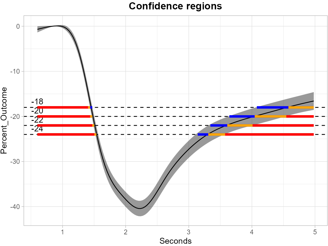
An Extended Example
Correlation and Multiplicity Adjusted (CMA) Confidence Bands
SCB for Mean Outcome Function
To further illustrate the power of
SCoRES::SCB_functional_outcome for constructing SCBs for
multiple group variables, we add age and gender as covariates, and
analyze the 40-year-old male user group by specifying
group_name = c("use", "age", "gender") and
group_value = c(1, 40, 0). We set
fitted = TRUE.
The function-on-scalar regression model is
pupil_fpca <- SCoRES::prepare_pupil_fpca(pupil, example = "extended")
fosr_mod <- mgcv::bam(percent_change ~ s(seconds, k=30, bs="cr") +
            s(seconds, by = use, k=30, bs = "cr") +
            s(seconds, by = age, k = 30, bs = "cr") +
            s(seconds, by = gender, k = 30, bs = "cr") +
            s(id, by = Phi1, bs="re") +
            s(id, by = Phi2, bs="re") +
            s(id, by = Phi3, bs="re") +
            s(id, by = Phi4, bs="re"),
            method = "fREML", data = pupil_fpca, discrete = TRUE)
The SCBs are estimated using both options separately for the mean outcome Y(t) of the specified group:
The following plots show the SCBs and inverse SCBs for the mean outcome function. The first one is from CMA approach and the second is from multiplier bootstrap.
# CMA approach
results_pupil_cma <- SCoRES::SCB_functional_outcome(
                                          data_df = pupil,
                                          object = fosr_mod,
                                          method = "cma",
                                          fitted = TRUE,
                                          alpha = 0.05,
                                          outcome = "percent_change",
                                          domain = "seconds",
                                          subset = c("use = 1",
                                                     "age = 40",
                                                     "gender = 0"),
                                          id = "id")

results_pupil_cma <- tibble::as_tibble(results_pupil_cma)
plot_cs(results_pupil_cma,
        levels = c(-18, -20, -22, -24),
        x = results_pupil_cma$domain,
        mu_hat = results_pupil_cma$mu_hat,
        xlab = "Seconds",
        ylab = "Percent_Outcome",
        level_label = T,
        min.size = 40,
        palette = "Spectral",
        color_level_label = "black")
Multiplier-t Bootstrap Confidence Bands
SCB for Mean Outcome Function
# Multiplier-t Bootstrap
results_pupil_multiplier <- SCoRES::SCB_functional_outcome(
                                          data_df = pupil,
                                          object = fosr_mod,
                                          fitted = TRUE,
                                          method = "multiplier",
                                          alpha = 0.05,
                                          outcome = "percent_change",
                                          domain = "seconds",
                                          subset = c("use = 1",
                                                     "age = 40",
                                                     "gender = 0"),
                                          id = "id")

results_pupil_multiplier <- tibble::as_tibble(results_pupil_multiplier)
plot_cs(results_pupil_multiplier,
        levels = c(-18, -20, -22, -24),
        x = results_pupil_multiplier$domain,
        mu_hat = results_pupil_multiplier$mu_hat,
        xlab = "Seconds",
        ylab = "Percent_Outcome",
        level_label = T,
        min.size = 40,
        palette = "Spectral",
        color_level_label = "black")